手撕Transformer Block：把Attention、FFN、Norm拼起来

前面几篇文章，我们已经把 Transformer Block 里的核心零件基本都手撕了一遍：

• Multi-Head Attention：让不同 Token 之间互相交流
• FFN：让每个 Token 独立做非线性加工
• 残差连接：把原始输入加回来，防止信息丢失
• LayerNorm：把数值拉回稳定范围

这一篇，我们不再单独看零件，而是把它们真正拼起来，写出一个最小版 Transformer Block。

---

一个 Block 到底长什么样？

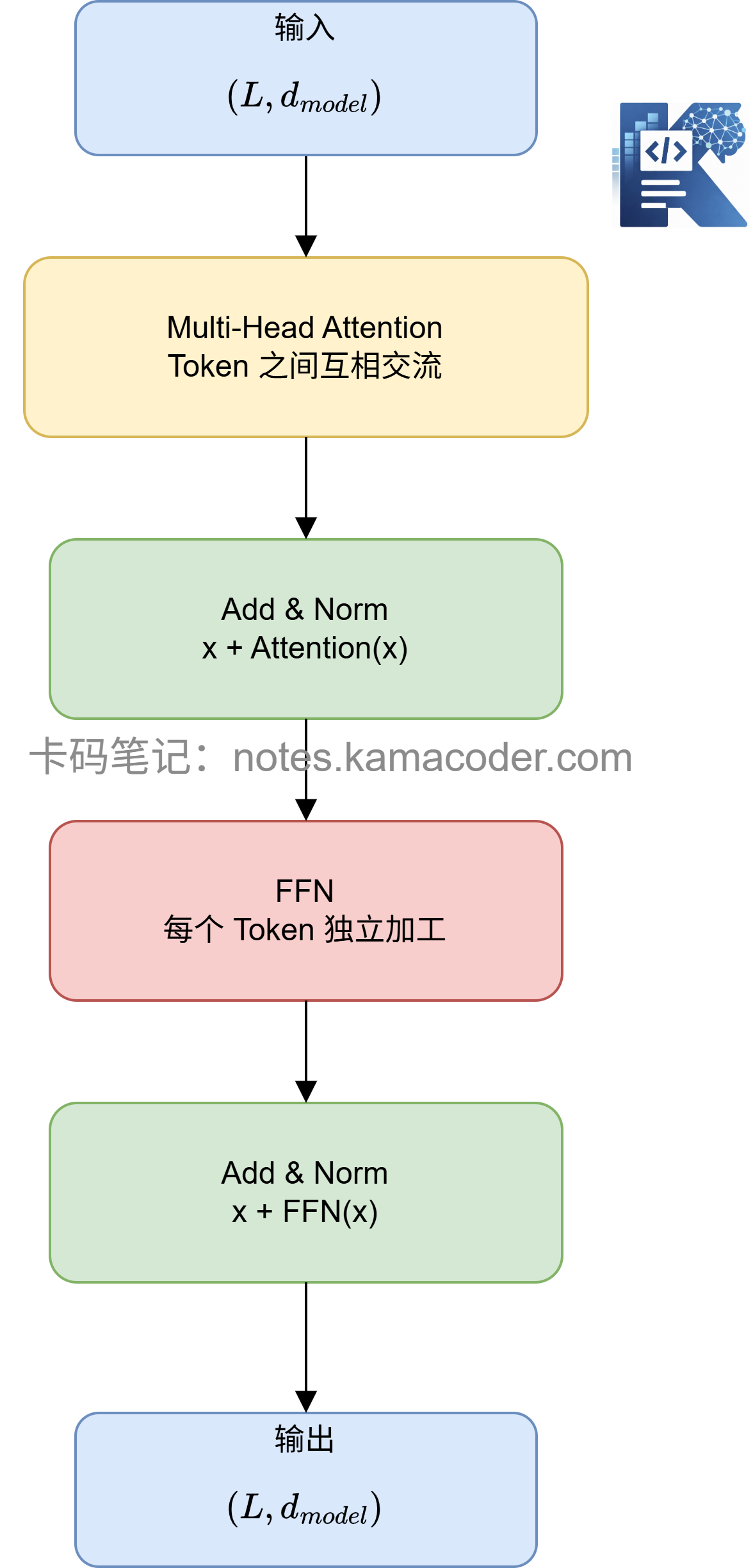
最常见的 Transformer Block 可以写成：

输入 x
  ↓
Multi-Head Attention
  ↓
残差连接 + LayerNorm
  ↓
FFN
  ↓
残差连接 + LayerNorm
  ↓
输出

也就是：

$$x_1 = \text{LayerNorm}(x + \text{MHA}(x))$$

$$x_2 = \text{LayerNorm}(x_1 + \text{FFN}(x_1))$$

这里有一个非常重要的点：

输入是什么形状，输出还是什么形状。

假设输入是：

x.shape = (L, d_model)

其中：

• L 是序列长度，比如“远方有颗苹果树”有 7 个 token
• d_model 是每个 token 的向量维度，比如这里用 8 维演示

那么经过一个 Transformer Block 后，输出仍然是：

output.shape = (L, d_model)

这也是为什么 Transformer 可以一层一层往上堆。

先写 LayerNorm 和 FFN

我们先把最基础的组件准备好。

import numpy as np

class LayerNorm:
    def __init__(self, d_model, eps=1e-5):
        self.gamma = np.ones(d_model)
        self.beta = np.zeros(d_model)
        self.eps = eps

    def forward(self, x):
        mean = x.mean(axis=-1, keepdims=True)
        std = x.std(axis=-1, keepdims=True)
        x_norm = (x - mean) / (std + self.eps)
        return self.gamma * x_norm + self.beta

LayerNorm 做的事很简单：对每个 Token 自己的向量做归一化。

比如输入是 (7, 8)，表示 7 个 token，每个 token 8 维，那么 LayerNorm 会分别对这 7 行做归一化。

接着写 FFN：

class FeedForward:
    def __init__(self, d_model, d_ff):
        self.W1 = np.random.randn(d_model, d_ff) * 0.01
        self.b1 = np.zeros(d_ff)
        self.W2 = np.random.randn(d_ff, d_model) * 0.01
        self.b2 = np.zeros(d_model)

    def gelu(self, x):
        return 0.5 * x * (1 + np.tanh(
            np.sqrt(2 / np.pi) * (x + 0.044715 * x ** 3)
        ))

    def forward(self, x):
        hidden = x @ self.W1 + self.b1
        hidden = self.gelu(hidden)
        output = hidden @ self.W2 + self.b2
        return output

FFN 的过程就是：

(L, d_model)
   ↓ 升维
(L, d_ff)
   ↓ GELU
(L, d_ff)
   ↓ 降维
(L, d_model)

还是那句话：中间怎么变都可以，但最后必须回到 d_model。

写 Multi-Head Attention

现在写一个最小版多头注意力。

class MultiHeadAttention:
    def __init__(self, d_model, num_heads):
        assert d_model % num_heads == 0

        self.d_model = d_model
        self.num_heads = num_heads
        self.d_k = d_model // num_heads

        self.W_Q = np.random.randn(d_model, d_model) * 0.01
        self.W_K = np.random.randn(d_model, d_model) * 0.01
        self.W_V = np.random.randn(d_model, d_model) * 0.01
        self.W_O = np.random.randn(d_model, d_model) * 0.01

    def softmax(self, x):
        e = np.exp(x - np.max(x, axis=-1, keepdims=True))
        return e / e.sum(axis=-1, keepdims=True)

    def split_heads(self, x):
        L, d_model = x.shape
        return x.reshape(L, self.num_heads, self.d_k).transpose(1, 0, 2)

    def forward(self, x):
        L, d_model = x.shape

        Q = x @ self.W_Q
        K = x @ self.W_K
        V = x @ self.W_V

        Q = self.split_heads(Q)
        K = self.split_heads(K)
        V = self.split_heads(V)

        head_outputs = []

        for i in range(self.num_heads):
            scores = Q[i] @ K[i].T / np.sqrt(self.d_k)
            weights = self.softmax(scores)
            out = weights @ V[i]
            head_outputs.append(out)

        concat = np.stack(head_outputs, axis=0)
        concat = concat.transpose(1, 0, 2).reshape(L, d_model)

        output = concat @ self.W_O
        return output

这里最容易绕的还是 shape：

输入 x:              (L, d_model)
Q/K/V:               (L, d_model)
拆成多个头:          (num_heads, L, d_k)
每个头输出:          (L, d_k)
拼接回来:            (L, d_model)
输出投影后:          (L, d_model)

可以看到，Attention 虽然中间拆成多个头，但最后依然回到原来的形状。

---

定义完整 Transformer Block

现在核心来了。

class TransformerBlock:
    def __init__(self, d_model, num_heads, d_ff):
        self.attn = MultiHeadAttention(d_model, num_heads)
        self.ffn = FeedForward(d_model, d_ff)

        self.norm1 = LayerNorm(d_model)
        self.norm2 = LayerNorm(d_model)

    def forward(self, x):
        print(f"输入 x:              {x.shape}")

        attn_out = self.attn.forward(x)
        print(f"Attention 输出:      {attn_out.shape}")

        x = self.norm1.forward(x + attn_out)
        print(f"Add & Norm 之后:     {x.shape}")

        ffn_out = self.ffn.forward(x)
        print(f"FFN 输出:            {ffn_out.shape}")

        x = self.norm2.forward(x + ffn_out)
        print(f"Block 最终输出:      {x.shape}")

        return x

这就是一个最小版 Transformer Block。

注意这里用了 Post-Norm 写法：

x = norm(x + sublayer(x))

也就是先经过子层，再残差相加，最后 LayerNorm。

现代很多大模型会使用 Pre-Norm：

x = x + sublayer(norm(x))

但为了和原始 Transformer 结构更一致，也为了方便初学者理解，这里先用 Post-Norm。

---

跑通一个 toy example

我们继续用熟悉的句子：

远方有颗苹果树

假设它被切成 7 个 token，每个 token 用 8 维向量表示。

if __name__ == "__main__":
    np.random.seed(42)

    L = 7
    d_model = 8
    num_heads = 2
    d_ff = 32

    x = np.random.randn(L, d_model)

    block = TransformerBlock(
        d_model=d_model,
        num_heads=num_heads,
        d_ff=d_ff
    )

    output = block.forward(x)

    print("\n=== 检查结果 ===")
    print("输入形状:", x.shape)
    print("输出形状:", output.shape)
    print("形状一致:", x.shape == output.shape)

运行输出大概是：

输入 x:              (7, 8)
Attention 输出:      (7, 8)
Add & Norm 之后:     (7, 8)
FFN 输出:            (7, 8)
Block 最终输出:      (7, 8)

=== 检查结果 ===
输入形状: (7, 8)
输出形状: (7, 8)
形状一致: True

这说明我们的最小版 Transformer Block 已经跑通了。

从输入到输出，形状始终保持 (7, 8)。

但是注意：形状没变，不代表内容没变。

经过 Attention 之后，每个 Token 已经融合了其他 Token 的上下文信息。

经过 FFN 之后，每个 Token 又单独做了一次非线性加工。

再加上残差连接和 LayerNorm，整个 Block 就既能表达复杂语义，又能保持训练稳定。

---

总结

一个 Transformer Block 本质上就是：

先让 Token 之间交流，
再让每个 Token 自己思考，
每一步都用残差保留原信息，
再用 LayerNorm 稳定数值。

如果再压缩成代码，就是这两行：

x = norm1(x + attention(x))
x = norm2(x + ffn(x))

这就是 Transformer Block 的核心。

看起来简单，但大模型就是把这样的 Block 堆几十层、上百层，再配上海量数据和算力训练出来的。

下一篇文章将继续带大家从 0 拼一个 Tiny Transformer，大家可以点个关注不迷路哦~